Overview
In order to conditionally hiding rows, conditionally hiding columns or conditionally hiding sheets automatically, you can include the HIDE keyword in the first cell of the column or row you want to hide:

Once a report has run, you can always hide a worksheet by using the keyword AUTO+HIDE+HIDESHEET in cell A1 of that worksheet.
Occasionally, you may want to hide entire rows, columns, or even worksheets all based on some criteria that may or may not be present. This is referred to as Conditional Hiding.
👉 Join our Jet Reports Training and learn to create real-time, dynamic reports with confidence.
Conditionally hiding Rows
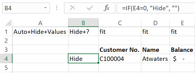
1) Place HIDE+? in cell B1.

2) Use formula to return Hide in column B of any row you want hidden.
In this example, let’s hide any row where the Balance (in column E) is equal to zero.
3) When we run the report…

We see that there are no zero balances and we can see that rows 4-10, 12-14, and 19 have been hidden.
Conditionally hiding Column
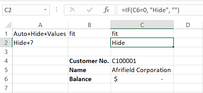
1) Place HIDE+? in cell A2
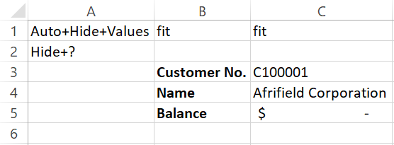
2) Use a formula to return Hide in row 2 of any column we want to hide.
In this example, we will hide the column if the Balance (in row 6) is equal to zero.
3) When we run the report…

We see that there are no zero balances and we can see that columns C-I and K-M have been hidden
.
Conditionally hiding Sheets
Similar to hiding a column, you can also hide an entire sheet.
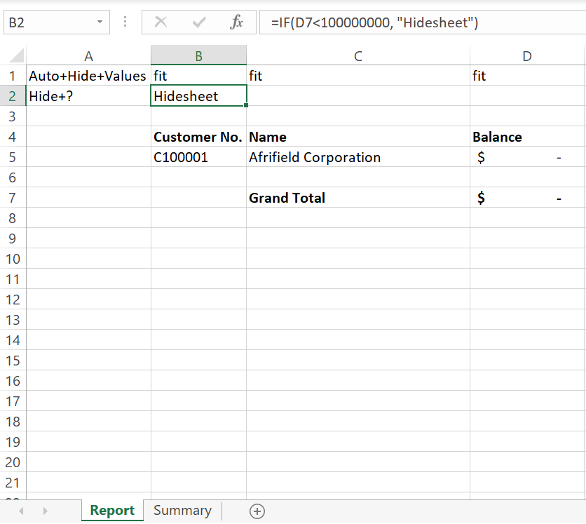
1) Place HIDE+? in cell A2

2) Use a formula to return HideSheet in cell B2 if our condition is met.
In this example, let’s hide the worksheet if the Grand Total (in cell D7) is less than a particular amount.
3) When we run the report…
We see that the entire Report sheet has been hidden with conditionally hiding rows, columns or sheets. This guide shows you precisely how jet reports conditional hide works.
Find and learn more about: Jet Reports with Global Data 365.


